4 minute read · Free exercise
12 Excel Shortcuts for Cleaning Up a Messy Export
A messy export usually needs a short routine: check its shape, make it readable, find the relevant rows and add a helper column. You can do much of that with a handful of keyboard commands.
This guide uses Excel desktop on Windows. Follow it on a copy of the practice export; the printable reference contains the same twelve shortcuts.
The five-step routine: make a Table with Ctrl+T, toggle filters with Ctrl+Shift+L, fill a checked formula with Ctrl+D, format with Ctrl+1, and return to the start with Ctrl+Home.
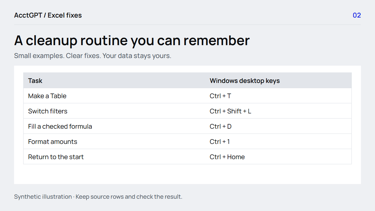
1. Save a working copy, then make a Table
Keep the downloaded original. Open a copy with a useful name such as monthly-expenses-working.xlsx and press Ctrl+S to save it. If you need a new filename, use File → Save As first; Ctrl+S saves the current file.
Click inside the data and press Ctrl+T. Check the proposed range before accepting it. If the first row contains column names, select My table has headers.
A blank row can split an export into separate regions. Look at the first and last rows of the selected range rather than assuming Excel included everything. In the six-row practice export, all six data rows should be inside the Table.
2. Find and filter the rows that matter
Press Ctrl+F to find a known ID or category. This is a useful first check when a total looks wrong: confirm the source row actually exists before changing a formula.
Use Ctrl+Shift+L to toggle the filter buttons for a selected range. Tables already have filters; the same shortcut can toggle them. With a header selected, Alt+Down Arrow opens its filter choices.
After filtering, the visible rows are a subset. Keep the full-file row count and total separate from the filtered view. If you need a visible-row total, the formula guide explains SUBTOTAL.
3. Move and select without losing your place
Use Ctrl+Arrow to move to the edge of a data region. Use Ctrl+Shift+Arrow to extend a selection along that route. These are useful when a column contains hundreds of rows, but blanks change where the movement stops.
Try both on a column with an intentional blank, then on a complete column. The result makes the rule easier to remember than a description alone.
Press Ctrl+Home to return to the start of the sheet. It is a reliable way to get back to the headers after inspecting the bottom of an export.
4. Edit and fill one checked formula
Select a formula cell and press F2 to edit it. On some laptops, the function key setting means you need Fn+F2.
First prove the formula on one row. Then select that cell and its intended destinations and press Ctrl+D to fill down from the top cell. Check that relative references moved and fixed references stayed fixed.
For this routine, clear filters before filling the full helper column. Filling only visible cells is a separate task and needs a deliberately selected visible-only range. A fast command is useful only when the selected cells are the ones you intended.
5. Format the meaning, then check what changed
Press Ctrl+1 to open Format Cells. Use a number format for amounts, a date format for actual dates and text for identifiers that need leading zeros.
Formatting a number as currency does not convert a text value into a number. Changing a code's display does not recover an original code that was already shortened. Check the underlying value when the format and result disagree.
If the last change was wrong, Ctrl+Z undoes it. Confirm the result rather than pressing Undo repeatedly without knowing which operation it is reversing.
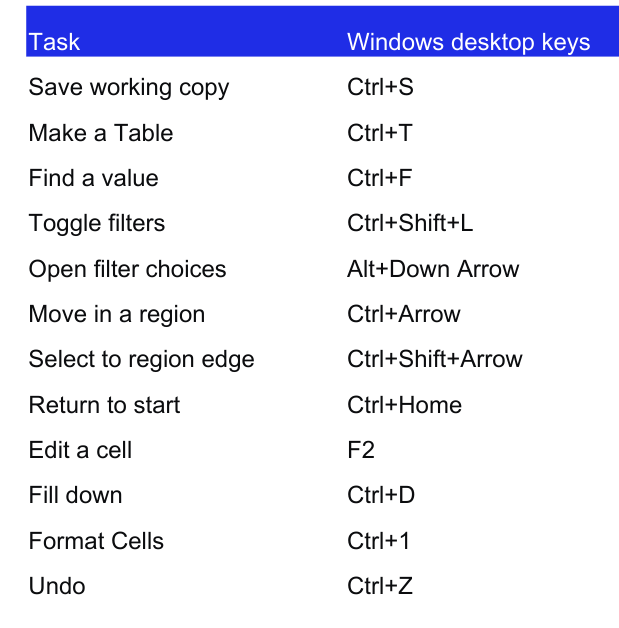
The twelve-command reference
| Job | Windows desktop shortcut |
|---|---|
| Save the current working file | Ctrl+S |
| Create a Table from the selected range | Ctrl+T |
| Find a value | Ctrl+F |
| Toggle filter buttons | Ctrl+Shift+L |
| Open choices for the selected filter header | Alt+Down Arrow |
| Move to a data-region edge | Ctrl+Arrow |
| Extend the selection to a region edge | Ctrl+Shift+Arrow |
| Return to the start | Ctrl+Home |
| Edit the active cell | F2 |
| Fill down from the top selected cell | Ctrl+D |
| Open Format Cells | Ctrl+1 |
| Undo the last reversible action | Ctrl+Z |
The Microsoft keyboard reference has separate Windows, Mac and web guidance. This reference is deliberately labelled for Windows; browser and Mac commands can differ.
Finish the practice run by checking that six source rows remain, your helper formula covers the intended rows and the amount total still agrees with the original. There is no need to memorize all twelve at once. Keep the reference beside the next export and use the command that solves the next step.
Watch the check
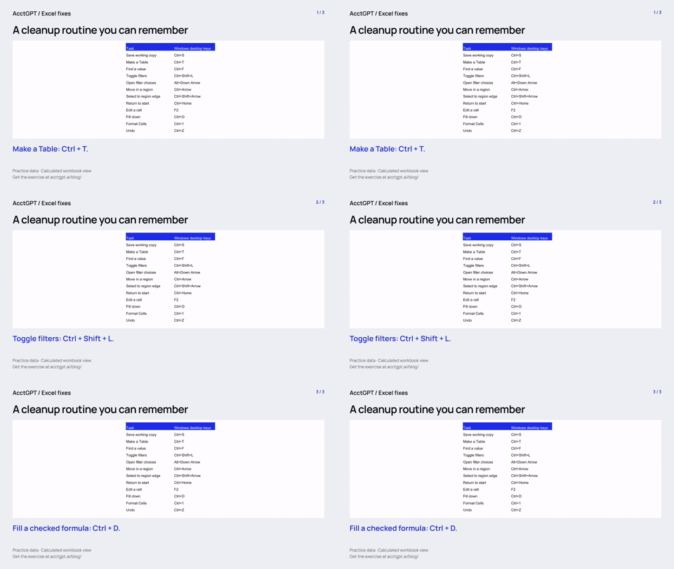
Read the animation
- Make a Table: Ctrl + T.
- Toggle filters: Ctrl + Shift + L.
- Fill a checked formula: Ctrl + D.
Calculated practice values, shown as a short visual explanation. No narration or recording of Excel menu actions.
Try it on a small example
Use the synthetic exercise first, check its expected answers, then adapt a copy for your own work.
Free files, no signup. Separate from the invitation-only $5 reporting kit.
Compatibility and example checks
The main walkthrough targets Excel desktop on Windows. Confirm each Mac equivalent against Microsoft's Mac tab and record it separately before publication. Do not label Windows ribbon sequences as universal.
The workbook’s formulas and source-edit/PivotTable refresh were checked with LibreOffice 26.8. Native Microsoft Excel editing, menu actions and Power Query execution are not yet verified for this release. The guide links to Microsoft’s instructions. The animations illustrate calculated examples rather than recording Excel actions.