4 minute read · Free exercise
7 Excel Formulas That Fix Everyday Spreadsheet Problems
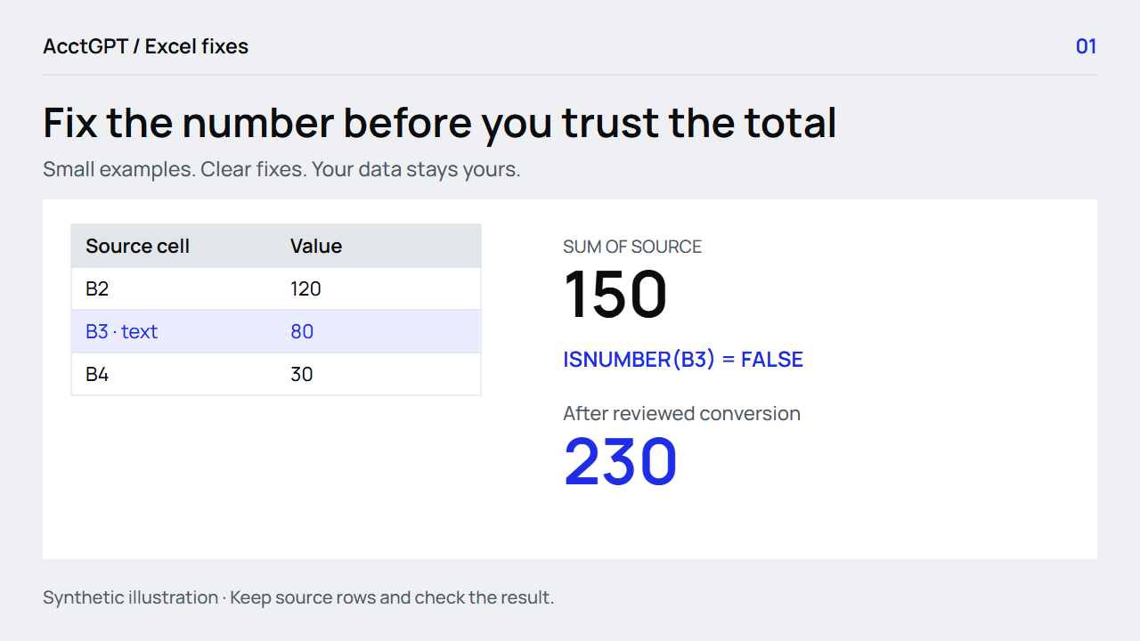
You have three amounts: 120, 80 and 30. Excel shows a total of 150. The missing 80 is sitting in a cell as text.
The quickest fix is to check the input, correct a copy and compare the result. The practice workbook below lets you reproduce the problem and try seven useful Excel formulas on small examples.
Start here: enter =ISNUMBER(B3) beside the suspect amount. FALSE means the cell is not a number. Keep the source value, convert a reviewed copy, and check the new total: 230.
1. ISNUMBER: find an amount stored as text
Open the Formulas sheet in the free workbook. B2 contains the number 120, B3 contains the text 80, and B4 contains the number 30. A normal range sum ignores the text cell:
=SUM(B2:B4)
The answer is 150. In a helper column, check each source cell:
=ISNUMBER(B3)
That check returns FALSE for B3. On a working copy, use Excel's Convert to Number warning option when appropriate. If the text uses currency symbols or unfamiliar separators, confirm the convention before converting it. A comma can mean a decimal separator in one export and a thousands separator in another.
The reviewed numeric column in the example totals 230. Keep the original beside it so the correction remains understandable. An identifier such as 00042 should remain text; being made of digits does not make a value an amount.
2. SUMIFS: add the rows that belong in the answer
Suppose your question is “How much did General expenses total in November?” Adding the whole amount column can include another category or month.
The workbook has a Table named Transactions. With the month starting in A2, use:
=SUMIFS(Transactions[Amount],
        Transactions[Category],"General",
        Transactions[Date],">="&A2,
        Transactions[Date],"<"&EDATE(A2,1))
Set A2 to the real date 1 November 2026. The three example expenses, 800, 350 and 200, return 1,350. The lower bound includes the first day; the upper bound stops before the next month. This also handles dates that carry a time of day.
Read the formula as “sum Amount where the category and both date conditions match.” Microsoft's SUMIFS reference explains the argument order.
3. COUNTIFS: flag a repeated combination
In the Duplicates sheet, invoice 002 appears twice with an amount of 250. To flag rows where both the ID and amount repeat, use:
=COUNTIFS($A$2:$A$4,A2,$B$2:$B$4,B2)>1
The two 002/250 rows return TRUE. The 001/100 row returns FALSE. The dollar signs keep the comparison ranges fixed when you fill down.
Choose the fields that define one record. A repeated invoice ID may be a legitimate second line item. A flag means review these rows; it is not a deletion instruction. For a repeated ID regardless of amount, use COUNTIF on the ID column instead.
4. SUBTOTAL: total the rows you can see
Filtering a list changes what is visible, but a normal SUM still includes filtered-out numeric rows. To total the visible numeric values, use:
=SUBTOTAL(109,D2:D4)
In the reviewed numeric example, all three rows give 230. Filter the source table and watch which rows contribute. The code 109 selects SUM and excludes filtered-out and manually hidden rows. Label this number Visible total so it is not mistaken for the full-file control total.
5. IF: make the review decision readable
A TRUE/FALSE helper is useful while building a sheet. A clear label is easier for someone reviewing it later:
=IF(COUNTIF($A$2:$A$4,A2)>1,"Review repeated ID","OK")
Keep the condition visible in the formula and the source rows beside it. Avoid labels such as “bad transaction” when the only evidence is a repeated key.
6. IFERROR: show a useful fallback
If B2 is an amount and C2 is a quantity, division fails when the quantity is zero. A visible fallback is more useful than a silent zero:
=IFERROR(B2/C2,"Review quantity or amount")
For 100 divided by 4, the result is 25. For 100 divided by 0, the message tells you what to inspect. IFERROR catches several error types, so use it where that broad fallback is intentional. For a missing lookup specifically, IFNA can leave unrelated errors visible.
7. ROUND: state the precision you need
For a two-decimal reporting calculation:
=ROUND(10/3,2)
The result is 3.33. Keep source precision where it matters, and distinguish rounding a calculation from simply displaying fewer decimal places. Do not use a rounding rule to hide an unexplained difference.
Check the result before using it
The seven formulas serve different jobs: check a type, select rows, count a combination, total a filtered view, label a condition, handle an error and apply precision. Start with the question you need answered.
Download the workbook, open Formulas, and reproduce the 150 versus 230 check first. Then try the Budget, Duplicates and Checks sheets. These examples use English function names and commas; your Excel locale may use translated names and semicolons.
For more functions, Microsoft's function directory is a useful reference. If your first task is preparing the export, combine and tidy a list privately before adding formulas.
Watch the check
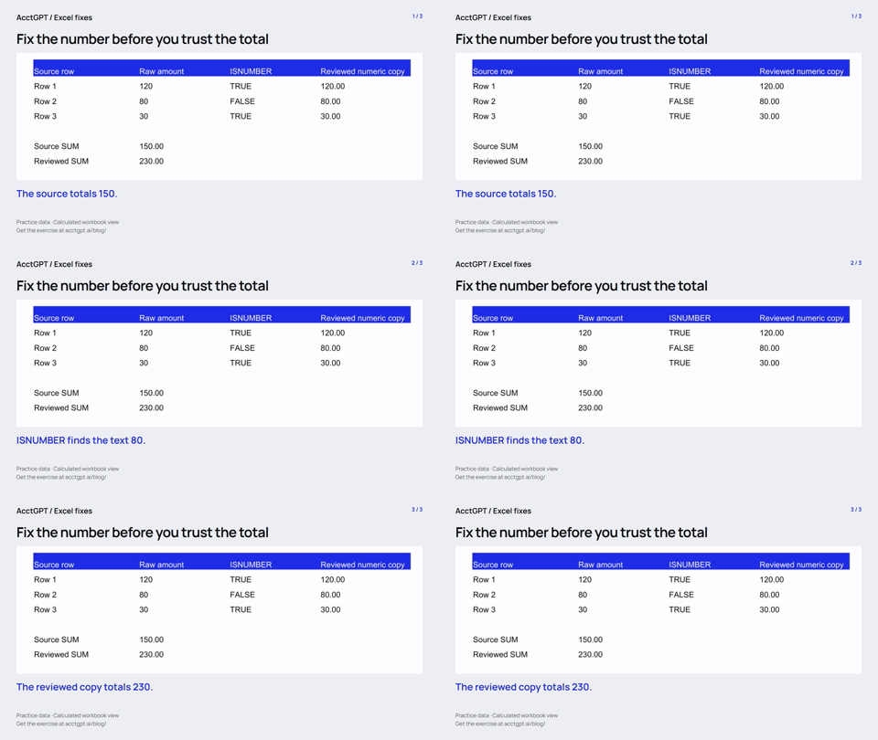
Read the animation
- The source totals 150.
- ISNUMBER finds the text 80.
- The reviewed copy totals 230.
Calculated practice values, shown as a short visual explanation. No narration or recording of Excel menu actions.
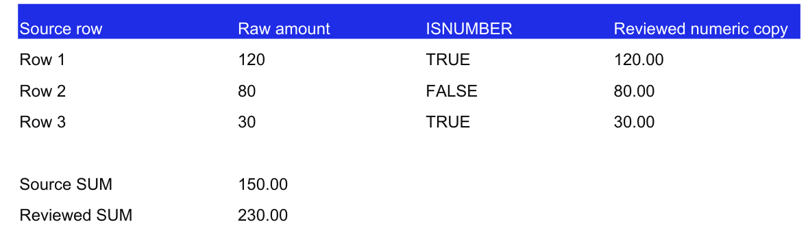
Try it on a small example
Use the synthetic exercise first, check its expected answers, then adapt a copy for your own work.
Free files, no signup. Separate from the invitation-only $5 reporting kit.
Compatibility and example checks
These seven functions work in Excel 2016 and later. Use English function names and comma separators in the examples; localized Excel may use translated names and semicolons.
The workbook’s formulas and source-edit/PivotTable refresh were checked with LibreOffice 26.8. Native Microsoft Excel editing, menu actions and Power Query execution are not yet verified for this release. The guide links to Microsoft’s instructions. The animations illustrate calculated examples rather than recording Excel actions.