4 minute read · Free exercise
Create a Pivot Table That Shows Where the Money Went
You have a list of expenses and need one answer: how much went to each category? A PivotTable can turn the rows into that summary without another set of hand-entered totals.
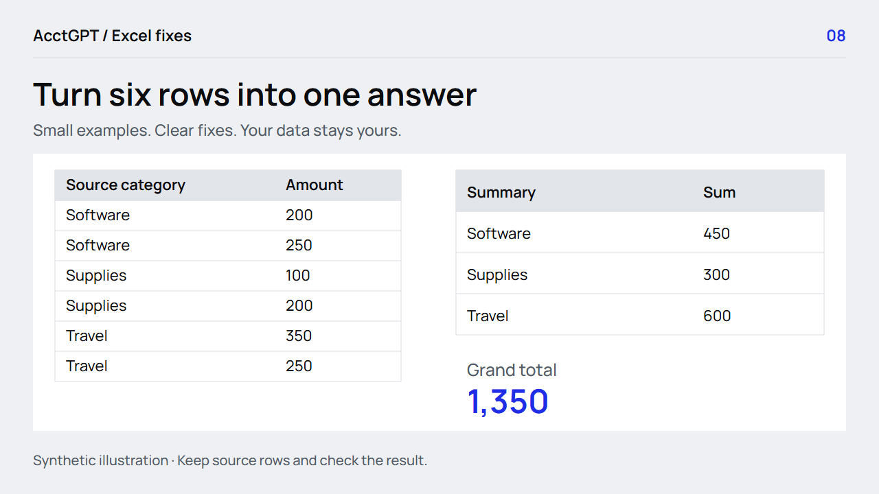
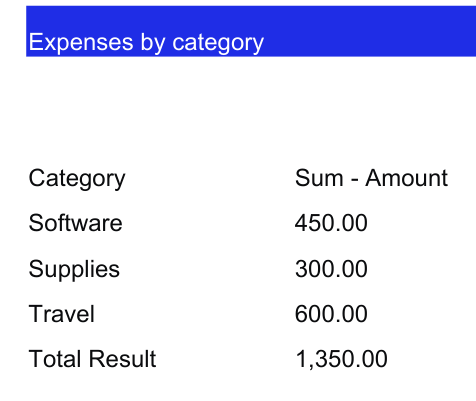
The exercise uses six expenses. Software totals 450, Supplies 300 and Travel 600, giving a grand total of 1,350.
Make the source an Excel Table, insert a PivotTable, put Category in Rows and Amount in Values, and confirm it uses Sum. Then check the grand total against the source.
1. Start with a clean source
Open PivotSource in the free workbook:
| Category | Amount |
|---|---|
| Software | 200 |
| Software | 250 |
| Supplies | 100 |
| Supplies | 200 |
| Travel | 350 |
| Travel | 250 |
Use one header row, no merged header cells, numeric amounts and consistent category names. This example represents one currency; keep currencies separate in a real report.
The source is already an Excel Table named Expenses. To build your own, click inside the range, press Ctrl+T, confirm the selected cells and check My table has headers. A Table makes the source easier to extend than a fixed range that stops at last month's final row.
2. Insert the PivotTable and place two fields
Click inside the source Table, then choose Insert → PivotTable → From Table/Range. Confirm the Table name and choose a new worksheet as the destination.
In the field list:
- Drag Category to Rows.
- Drag Amount to Values.
- Confirm the values field reads Sum of Amount, or an equivalent sum label.
Your summary should show 450, 300 and 600. The workbook also includes a working PivotTable on PivotSummary, so you can compare it with the one you create.
Microsoft's PivotTable instructions show the field list and the menu differences between platforms.
3. If it says Count of Amount, check the data
Count answers “how many records?” Sum answers “how much?” In this exercise, a category count of two is not the same answer as a category expense total of 450.
If Excel selected Count, inspect the source Amount column. Text amounts, blanks or inconsistent types can change how Excel interprets the field. Use a helper such as ISNUMBER to find suspect cells, correct a reviewed copy and refresh the PivotTable.
To select the calculation, open the values field's menu and choose Value Field Settings → Sum. Do not stop there if the original issue was a text amount: selecting Sum does not make every invalid source value numeric.
Use Number Format within Value Field Settings to apply the amount format to the values field, so the formatting follows the PivotTable as it changes.
4. Trace a category back to its rows
In desktop Excel, double-click a category's amount to extract the contributing detail into a new sheet. For Software, the two amounts are 200 and 250; together they explain 450.
Treat that extracted sheet as a snapshot. It is useful for checking the subtotal, but it does not become a new authoritative source or automatically stay synchronized with later changes.
When adapting the exercise to dates, filter the intended month explicitly. Use actual date values, and keep the date and currency scope visible in the report. The six-row exercise is deliberately small so the source remains easy to inspect.
5. Change a source value and refresh
On a working copy, change the first Software amount from 200 to 210. Refresh the PivotTable. Software should become 460, and the grand total should become 1,360.
Restore the source to 200 and refresh again. The expected total returns to 1,350. That checks more than the initial screenshot: it proves the PivotTable reads the source you intended.
Use PivotTable Analyze → Refresh, or right-click inside the PivotTable and choose Refresh. If adding new rows to a fixed source range, check Change Data Source as well. A refresh cannot include a row outside the defined range.
Refresh behavior varies by Excel version and connection. Newer versions can automatically refresh some local sources; older setups may need manual refresh or refresh-on-open settings. Microsoft's refresh guide describes those options.
Finish by confirming that the source sum and PivotTable grand total agree for the same filters. If the numbers differ, check source range, filters, value type and refresh state before rebuilding the report.
Download the exercise workbook and recreate the summary from PivotSource. Then turn the result into a small, checkable dashboard or use the file-combination guide when your source arrives in several exports.
Watch the check
Read the animation
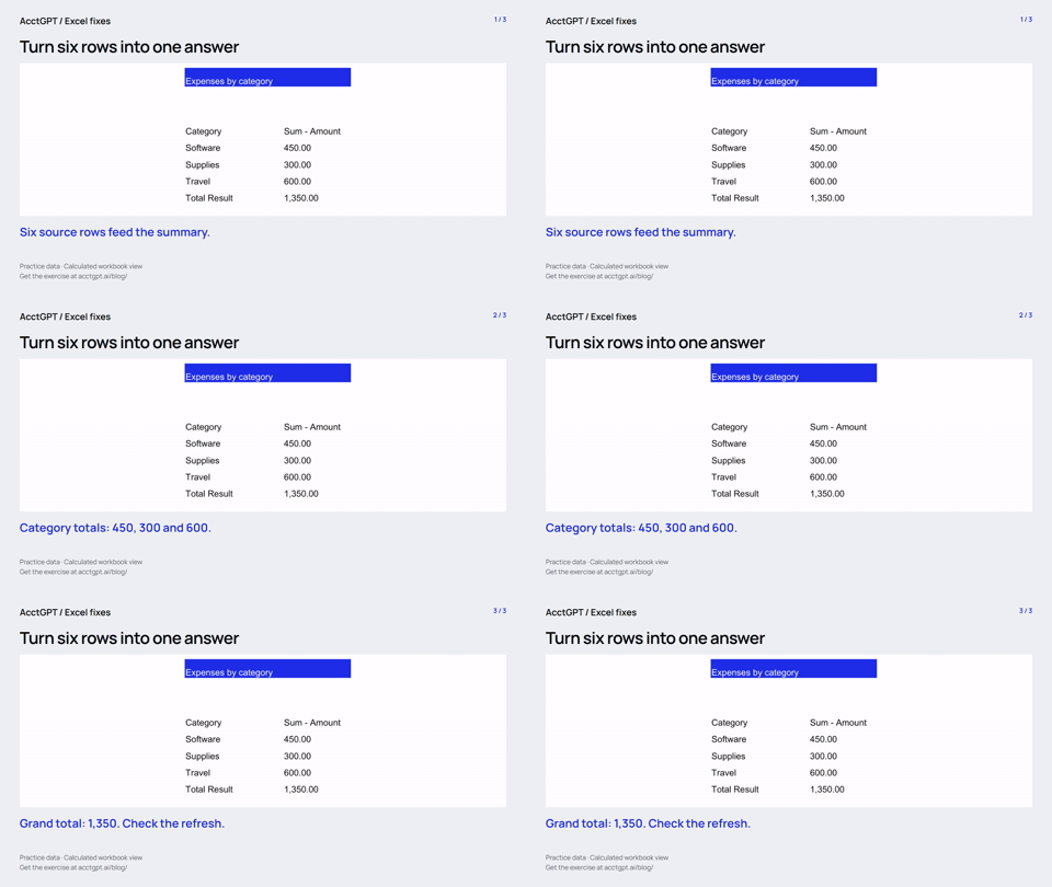
- Six source rows feed the summary.
- Category totals: 450, 300 and 600.
- Grand total: 1,350. Check the refresh.
Calculated practice values, shown as a short visual explanation. No narration or recording of Excel menu actions.
Try it on a small example
Use the synthetic exercise first, check its expected answers, then adapt a copy for your own work.
Free files, no signup. Separate from the invitation-only $5 reporting kit.
Compatibility and example checks
The walkthrough targets desktop Excel 2016 and later. Refresh options differ by version; newer Excel can auto-refresh some local sources, so demonstrate the actual refresh state rather than claiming every PivotTable is always manual.
The workbook’s formulas and source-edit/PivotTable refresh were checked with LibreOffice 26.8. Native Microsoft Excel editing, menu actions and Power Query execution are not yet verified for this release. The guide links to Microsoft’s instructions. The animations illustrate calculated examples rather than recording Excel actions.