4 minute read · Free exercise
Build an Excel Dashboard You Can Actually Check
A dashboard should help you decide what to inspect next. If you cannot explain where its biggest number came from, another chart will not solve the problem.
Start with one question: Which expense category needs attention this month? Then build a small summary whose total ties back to the source rows.
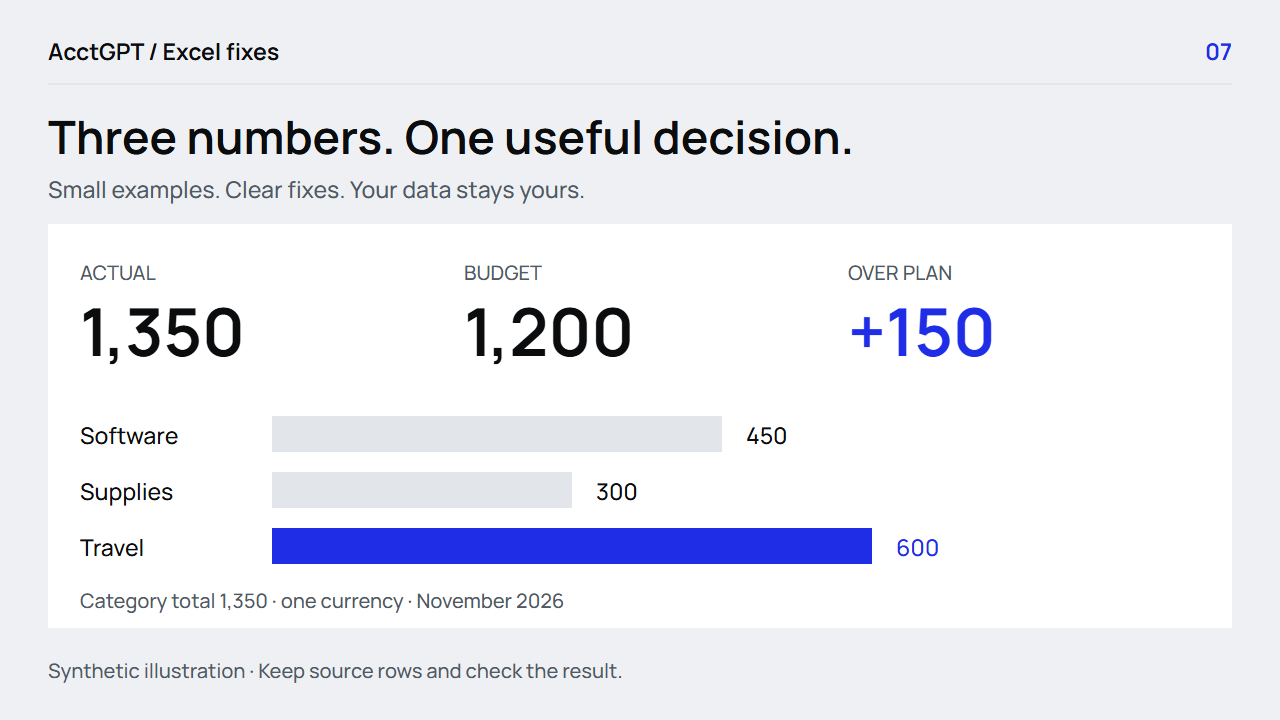
Use one clean source table, a few labelled measures and one chart. Keep the month, currency, source total and refresh context visible. The practice dashboard shows 1,350 actual expense against a 1,200 plan: 150 over plan.
1. Write the decision before drawing the dashboard
For this example, you need to see the category totals and decide which category to review. You do not need a world map, a gauge or twelve different chart types.
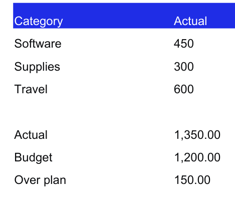
The workbook's Dashboard sheet has three categories: Software 450, Supplies 300 and Travel 600. Their total is 1,350. The underlying six rows are on PivotSource.
These are synthetic practice values in one currency. When replacing them, keep the period and currency explicit. A dashboard that combines different periods or currencies without a stated rule is hard to interpret, however polished it looks.
2. Establish a single source table
Use a Table with a clear header row and consistent fields. For an expense view, that usually means Date, Category, Currency and Amount, with a source reference when several exports are combined.
Before summarizing, check that amounts are numeric, categories are consistent and the date filter covers the intended month. Keep uncategorized or invalid rows in a visible review list rather than excluding them silently.
You can use a PivotTable or SUMIFS to build the summary. The PivotTable guide walks through a category summary; the budget guide shows date-bounded SUMIFS.
The supplied Dashboard uses a simple summary so you can inspect the numbers immediately. Its native chart uses those summary cells. If you adapt it into a recurring dashboard, link each measure to the appropriate source calculation instead of retyping numbers every month.
3. Define the measures in plain language
Start with these three:
| Measure | Meaning | Practice value |
|---|---|---|
| Actual expense | Included source expenses for the period | 1,350 |
| Budget | The spending plan for that same scope | 1,200 |
| Actual minus budget | Positive means over plan for expenses | +150 |
In the practice sheet, the summary is in B2:B4:
=SUM(B2:B4)
That actual total belongs in B6. With budget in B7, the variance in B8 is:
=B6-B7
If you add an “items to review” measure, define what counts as one item. A repeated ID group, a flagged source row and a missing category are different units. A meaningful label is more useful than a large unexplained red number.
4. Add one chart that answers the question
The supplied column chart compares the three category totals. It starts at zero and uses one clear measure. The category labels and numbers remain available in the table.
For your own version:
- Select the category labels and actual amounts.
- Choose Insert → Column or Bar Chart → Clustered Column.
- Give it a title that names the measure and period.
- Confirm the numeric axis starts at zero for this amount comparison.
- Keep the source summary visible beside or below it.
Use color to draw attention, then support it with a label or number. A reader should still understand the result in a grayscale printout. Microsoft also provides an Excel dashboard walkthrough for a broader PivotTable-based setup.
5. Show what is current and what needs action
Before sharing the view, check that the category totals add to 1,350 and that the same six source expenses also add to 1,350. Trace one category all the way back to its contributing rows.
For a recurring workbook, distinguish the latest source date from when the workbook was refreshed. A report can be refreshed today and still contain last month's data. A manual “last refreshed” note should only be changed after the refresh actually finishes.
If you use filters or slicers, reset them before comparing the dashboard with a full-file control total. A filtered subtotal is not a mismatch merely because it differs from the unfiltered total; the scope must match.
Finish with a specific review action, such as “inspect the Travel rows.” A high category total is a prompt to investigate, not proof that the spending was inappropriate.
Download the workbook and open Dashboard, PivotSource and PivotSummary. Together they show the measure, the rows and a second way to summarize them. If the source is still scattered across files, combine the exports privately or use the Power Query guide for a recurring Excel workflow.
Watch the check
Read the animation
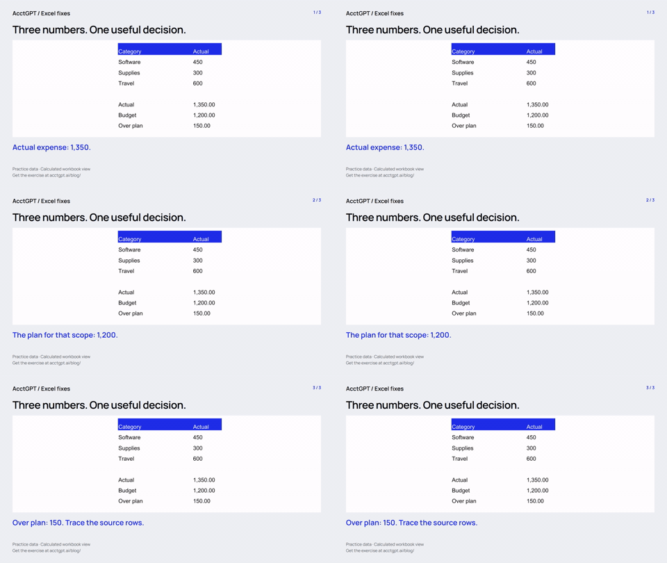
- Actual expense: 1,350.
- The plan for that scope: 1,200.
- Over plan: 150. Trace the source rows.
Calculated practice values, shown as a short visual explanation. No narration or recording of Excel menu actions.
Try it on a small example
Use the synthetic exercise first, check its expected answers, then adapt a copy for your own work.
Free files, no signup. Separate from the invitation-only $5 reporting kit.
Compatibility and example checks
The basic Tables, SUMIFS, PivotTable and column-chart version targets Excel 2016 and later. Capture slicer and refresh behavior in the chosen desktop version before advertising cross-platform support.
The workbook’s formulas and source-edit/PivotTable refresh were checked with LibreOffice 26.8. Native Microsoft Excel editing, menu actions and Power Query execution are not yet verified for this release. The guide links to Microsoft’s instructions. The animations illustrate calculated examples rather than recording Excel actions.